Central Forces: Spring-2026
HW 09 (SOLUTION): Due W5 D3

1. Sphere Table S1 5546S Attached, you will find a table showing different representations of physical quantities associated with a quantum particle confined to a sphere. Fill in all of the missing entries. Hint: You may look ahead. We filled out a number of the entries throughout the table to give you hints about what the forms of the other entries might be. pdf link for the Table or doc link for the Table

   pdf link for the completed Table

2. QM Sphere with Time Dependence S1 5546S Consider a quantum particle on a sphere. At t = 0, the particle is in state:\[\left|{\psi(t=0)}\right\rangle =\frac{1}{\sqrt{2}}\left(\left|{2,0}\right\rangle +\left|{1,0}\right\rangle \right)\] Calculate the following quantities for some later time, \(t>0\), and identify whether each quantity is time-dependent.
   1. \(\left|{\psi(t)}\right\rangle \).

      Each ket \(|\ell,m\rangle\) gets its own exponential energy term. The first ket has energy \(E_2=\frac{\hbar^2}{2I}\, 2(2+1)=6\frac{\hbar^2}{2I}\) and the second ket has energy \(E_1=\frac{\hbar^2}{2I}\, 1(1+1)=2\frac{\hbar^2}{2I}\). Therefore \[\left|{\psi(t)}\right\rangle =\frac{1}{\sqrt{2}}\left(\left|{2,0}\right\rangle e^{-iE_2t/\hbar} +\left|{1,0}\right\rangle e^{-iE_1t/\hbar}\right)\] This expression depends on time.

   2. \(\langle L_z\rangle\)

      Both kets, even as functions of time, are eigenstates of \(L_z\) with eigenvalue \(0\hbar\), therefore the expectation value is \(0\), independent of time.

      We can check that the calculation methods give this same answer:

      Using the sum over probabilities method, we see that \begin{align} \langle L_z\rangle&=0\hbar\, \mathcal{P}(\left|{2,0}\right\rangle )+0\hbar\, \mathcal{P}(\left|{1,0}\right\rangle )\\ &=0\hbar\,\left\vert\frac{1}{\sqrt{2}}\left|{2,0}\right\rangle e^{-iE_2t/\hbar}\right\vert^2 +0\hbar\,\left\vert\frac{1}{\sqrt{2}}\left|{1,0}\right\rangle e^{-iE_1t/\hbar}\right\vert^2\\ &=0\hbar\left(\frac{1}{2}+\frac{1}{2}\right)\\ &=0 \end{align}

      Using the bra/ket method, we see that \begin{align} \langle L_z\rangle &=\left\langle {\psi(t)}\right|\, L_z\, \left|{\psi(t)}\right\rangle \\ &=\frac{1}{\sqrt{2}}\left(\left\langle {2,0}\right|e^{iE_2t/\hbar} +\left\langle {1,0}\right|e^{iE_1t/\hbar}\right)\, L_z\,\frac{1}{\sqrt{2}}\left(\left|{2,0}\right\rangle e^{-iE_2t/\hbar} +\left|{1,0}\right\rangle e^{-iE_1t/\hbar}\right)\\ &=\frac{1}{\sqrt{2}}\left(\left\langle {2,0}\right|e^{iE_2t/\hbar} +\left\langle {1,0}\right|e^{iE_1t/\hbar}\right) \frac{1}{\sqrt{2}}\left(0\hbar\left|{2,0}\right\rangle e^{-iE_2t/\hbar} +0\hbar\left|{1,0}\right\rangle e^{-iE_1t/\hbar}\right)\\ &=0 \end{align}

   3. \(\mathcal{P}(L^2=6\hbar^2)\)

      The eigenvalue \(L^2=6\hbar^2\) corresponds to \(\ell=2\) which happens only for the first eigenket. \begin{align} \mathcal{P}(L^2=6\hbar^2)&=\left\vert\left\langle {2,0}\middle|{\psi(t)}\right\rangle \right\vert^2\\ &=\left\vert \frac{1}{\sqrt{2}}e^{-iE_2t/\hbar}\right\vert^2\\ &=\frac{1}{2} \end{align} The time dependence cancels. Any probability like this will cancel as long as the operator for which the physical property is being measured (in this case, \(L^2\)) commutes with the Hamiltonian. In that case, every eigenket has only one exponential time dependence in it and the time dependence will cancel for each separate probability.

   4. The probability that the particle can be found in the “southern” hemisphere.

      To calculate a probability in space, we need to use the wave function representation. We can look up the spherical harmonics in a table: \begin{align} \psi(\theta, \phi, t)&=\left\langle {\theta, \phi}\middle|{\psi(t)}\right\rangle \\ &=\frac{1}{\sqrt{2}}\left(Y_2^0(\theta,\phi)\, e^{-iE_2t/\hbar} +Y_1^0(\theta,\phi)\, e^{-iE_1t/\hbar}\right)\\ &=\frac{1}{\sqrt{2}}\left(\sqrt{\frac{5}{16\pi}}\left(3\cos^2\theta-1\right)\, e^{-iE_2t/\hbar} +\sqrt{\frac{3}{4\pi}}\left(\cos\theta\right)\, e^{-iE_1t/\hbar}\right)\\ \end{align} Now we need to integrate the probability density \(\vert\psi(t)\vert^2\) over the relevant part of the sphere. Don't forget to use the area element for the sphere (i.e. include a factor of \(\sin\theta\)). \begin{align} \mathcal{P}&=\int_0^{2\pi}\int_{\pi/2}^{\pi} \left[\frac{1}{\sqrt{2}}\left(\sqrt{\frac{5}{16\pi}}\left(3\cos^2\theta-1\right)\, e^{-iE_2t/\hbar} +\sqrt{\frac{3}{4\pi}}\left(\cos\theta\right)\, e^{-iE_1t/\hbar}\right)\right]^*\\ &\qquad\left[\frac{1}{\sqrt{2}}\left(\sqrt{\frac{5}{16\pi}}\left(3\cos^2\theta-1\right)\, e^{-iE_2t/\hbar} +\sqrt{\frac{3}{4\pi}}\left(\cos\theta\right)\, e^{-iE_1t/\hbar}\right)\right] \sin\theta\, d\theta\, d\phi\\ \end{align} Aaaackkk!! Don't panic. Take a deep breath, foil-like-mad, and recognize when you need to use the exponential definition of cosine: \begin{align} \mathcal{P}&=\frac{1}{2}\int_0^{2\pi}\int_{\pi/2}^{\pi} \left[\frac{5}{16\pi}\left(3\cos^2\theta-1\right)^2 +\frac{3}{4\pi}\left(\cos\theta\right)\right.\\ &\qquad\left.\sqrt{\frac{15}{64\pi^2}}\,\cos\theta\left(3\cos^2\theta-1\right)\, \left(e^{+iE_2t/\hbar}e^{-iE_1t/\hbar}+e^{+iE_1t/\hbar}e^{-iE_2t/\hbar}\right) \right] \sin\theta\, d\theta\, d\phi\\ &=\frac{1}{2}\int_0^{2\pi}\int_{\pi/2}^{\pi} \left[\frac{5}{16\pi}\left(3\cos^2\theta-1\right)^2 +\frac{3}{4\pi}\left(\cos\theta\right)\right.\\ &\qquad\left.\sqrt{\frac{15}{64\pi^2}}\,\cos\theta\left(3\cos^2\theta-1\right)\, 2\cos\left(\frac{(E_2-E_1)t}{\hbar}\right) \right] \sin\theta\, d\theta\, d\phi\\ \end{align} While this expression looks messy, it is the sum of a bunch of powers of \(\cos\theta\) times \(\sin\theta\), so a simple \(u\)-substitution will work. You can finish the problem.

      Because the cross-terms are non-zero, this expression will clearly be time dependent. The probability of where the mass is depends on time! Hurray! Finally the universe has become interesting.

   5. The probability that the particle can still (at the time \(t\)) be found in the state \[\left|{\psi}\right\rangle =\frac{1}{\sqrt{2}}\left(\left|{2,0}\right\rangle +\left|{1,0}\right\rangle \right)\]

      \begin{align} \mathcal{P}&=\left\vert\left\langle {\psi(0)}\middle|{\psi(t)}\right\rangle \right\vert^2\\ &=\left\vert\frac{1}{\sqrt{2}}\left(\left\langle {2,0}\right|+\left\langle {1,0}\right|\right) \frac{1}{\sqrt{2}}\left(\left|{2,0}\right\rangle e^{-iE_2t/\hbar} +\left|{1,0}\right\rangle e^{-iE_1t/\hbar}\right)\right\vert^2\\ &=\left\vert\frac{1}{2}\left(e^{-iE_2t/\hbar}+e^{-iE_1t/\hbar}\right)\right\vert^2\\ &=\frac{1}{4}\left(e^{iE_2t/\hbar}+e^{iE_1t/\hbar}\right) \left(e^{-iE_2t/\hbar}+e^{-iE_1t/\hbar}\right)\\ &=\frac{1}{4}\left(1+1 +\left(e^{+iE_2t/\hbar}e^{-iE_1t/\hbar}+e^{+iE_1t/\hbar}e^{-iE_2t/\hbar}\right)\right)\\ &=\frac{1}{2}\left(1+\cos\left(\frac{(E_2-E_1)t}{\hbar}\right)\right) \end{align} The state oscillates with time and returns to the initial state periodically.

3. Hydrogen, Version 1 S1 5546S

   A hydrogen atom is initially in the superposition state \begin{equation} \vert \psi(t=0) \rangle = \frac{1}{\sqrt{14}}\vert 2,1,1\rangle - \frac{2}{\sqrt{14}}\vert 3,2,-1\rangle + \frac{3}{\sqrt{14}}\vert 4,2,2\rangle . \end{equation}

   1. What are the possible results of a measurement of the energy and with what probabilities would they occur? Plot a histogram of the measurement results. Calculate the expectation value of the energy.

      The form of our answer should be a list of values for the quantity of interest (\(E\), \(L^2\), \(L_z\)) and the corresponding probabilities, which can also be presented in graphical form.

      The possible results of a measurement of energy correspond to the values of \(n\) represented in the superposition. These are \(n = 2,3,4\), where \(E_n = -13.6 eV/n^2\) The probabilities are found by taking appropriate inner products that collapse to the coefficients of the relevant terms, followed by taking the modulus square. \begin{eqnarray*} &{\cal P}_{E_2} = 1/14 \\ &{\cal P}_{E_3} = 4/14 \\ &{\cal P}_{E_4} = 9/14 \end{eqnarray*}

      
      

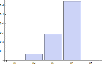
      The expectation value is the weighted average of the eigenvalues, which for this system gives:

      \(\langle E \rangle = -13.6 eV (1/14(1/4) + 4/14(1/9) + 9/14(1/16) = -13.6 eV (181/2016)\)

   2. What are the possible results of a measurement of the angular momentum operator \(L^2\) and with what probabilities would they occur? Plot a histogram of the measurement results. Calculate the expectation value of \(L^2\).

      The possible results of a measurement of \(L^2\) correspond to the values of \(\ell\) represented in the superposition. These are \(\ell = 1,2\), where \(L^2 = \hbar^2\ell(\ell+1)\) The probabilities are found by taking appropriate inner products that collapse to the coefficients of the relevant terms, followed by taking the modulus square. Because the superposition contains more than one term with the same value of \(\ell\), it is necessary to sum probabilities corresponding to degenerate states. \begin{eqnarray*} &{\cal P}_{2\hbar^2} = 1/14 \\ &{\cal P}_{6\hbar^2} = 13/14 \end{eqnarray*}

      
      

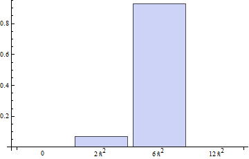
      The expectation value is the weighted average of the eigenvalues, which for this system gives:

      \(\langle L^2 \rangle = 1/14(2\hbar^2) + 13/14(6\hbar^2) = 40\hbar^2/7\)

   3. What are the possible results of a measurement of the angular momentum component operator \(L_z\) and with what probabilities would they occur? Plot a histogram of the measurement results. Calculate the expectation value of \(L_z\).

      The possible results of a measurement of \(L_z\) correspond to the values of \(m\) represented in the superposition. These are \(m = -1,1,2\), where \(L_z = \hbar m\) The probabilities are found by taking appropriate inner products that collapse to the coefficients of the relevant terms, followed by taking the modulus square. \begin{eqnarray*} &{\cal P}_{-\hbar} = 4/14 \\ &{\cal P}_{\hbar} = 1/14 \\ &{\cal P}_{2\hbar} = 9/14 \end{eqnarray*}

      
      

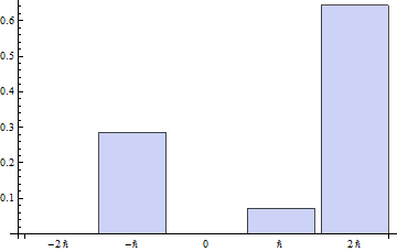
      The expectation value is the weighted average of the eigenvalues, which for this system gives:

      \(\langle L_z \rangle = 5/14(-\hbar) +1/14\hbar + 9/14(2\hbar) = 15\hbar/14\)

   4. How do the answers to (a), (b), and (c) depend upon time?

      Since the operators \(L_z\), \(L^2\) and \(H\) itself all commute with the Hamiltonian, none of the previous answers will depend on time.