Theoretical Mechanics: Fall-2026
HW 0 (SOLUTION): Due F Day 3 MathBits
- Intro to Ph335 Email
S1 5341S
Fill out the online survey at:
https://beav.es/xex
- Obtain Plotting Software
S1 5341S
In this course, you will be asked to plot functions using either Mathematica, Matlab, or Python. The university has a license that allows undergraduate students to download and use these computer algebra systems on their personal computers, but you have to send an e-mail to receive an access code:
for Mathematica: https://softwarelist.oregonstate.edu/software/mathematica (Link on Canvas Too)
for Matlab: https://softwarelist.oregonstate.edu/software/matlab (Link on Canvas Too)
for Python: https://www.anaconda.com/products/individual (Link on Canvas Too)
(There's nothing to turn in for this problem. This is just to prepare you for future homework.)
Needing help getting any or all of the above software working is a perfectly good reason to come to office hours.
Rules for Plots in this Course:
- Use a Computer - you may use Mathematica, Wolfram Alpha, Matlab, or Python. The physics faculty like for you to be familiar with more powerful computational software - it will be useful skill to have in later physics classes and beyond. Mathematica is my preferred choice.
- Plot Caption - describe your plot so that the reader knows what it is.
- Parameters - indicate the value of all parameters chosen.
- Axis Labels - make sure the axes are labeled and indicate the units of quantities.
- Font Size - make sure that all font sizes are large enough to be easily read.
- Domain and Range - choose appropriate domain (horizontal axes) and range (vertical axis).
- the domain should include all relevant values (but no more)
- the range and scale should be chosen so that the graph is interpretable (interesting features should be noticeable).
- the range should start from zero unless that makes the interesting functional behavior interesting to see.
- Labeling Functions -different functions should be visually distinguishable (in printed form, using different colors or line styles) and labeled or indicated in a legend.
- Interpret -always interpret your graph with words or diagrams with respect to the physical situation.
- Code - always indicate which plotting software you used and include the code you used to generate the plot .
For help with plotting in Mathematica, see:
- Basic Plotting
http://reference.wolfram.com/language/tutorial/BasicPlotting.html
- Plot Functions of One Variable
http://reference.wolfram.com/language/howto/PlotFunctionsOfOneVariable.html
- Plot
http://reference.wolfram.com/language/ref/Plot.html
- Customize Plots and Graphics
http://reference.wolfram.com/language/howto/CustomizePlotsAndGraphics.html
- Intro to Hyperbolic Trig
S1 5341S
(modified from Taylor 2.33 & 2.34)
Hyperbolic trigonometry is going to be useful for us both for describing the motion of objects experiencing quadratic drag force and also for geometric approaches to special relativity. You should be familiar with the properties of these hyperbolic trig functions for later parts of this course.
The hyperbolic functions \(\cosh z\) and \(\sinh z\) are defined as follows: \begin{align} \cosh z &= \frac{e^z+e^{-z}}{2} \\ \sinh z &= \frac{e^z-e^{-z}}{2} \\ \end{align}
for any \(z\), real or complex.
- Plot the behavior of \(\cosh z\) and \(\sinh z\) over a suitable range of real values z. Describe the behavior of these functions in words and note what the values of the functions are near \(z=0\) and \(z=\pm \infty\).
First, I'll plot \(\cosh(z)\) vs. \(z\)
At \(z=0\), I get \(\cosh(0) = 1\) and
at \(z=\pm\infty\), I get \(\cosh(\pm\infty) = +\infty\).
\(\cosh z\) is even: \(\cosh(-z)=\cosh)z)\).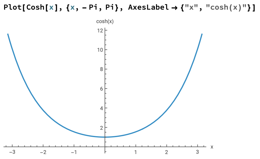
Now, I plot \(\sinh(z)\) vs. \(z\)
At \(z=0\), I get \(\sinh(0) = 0\) and
at \(z=\pm\infty\), I get \(\sinh(\pm\infty) = \pm\infty\).
\(\sinh z\) is odd: \(\sinh(-z)=-\sinh(z)\)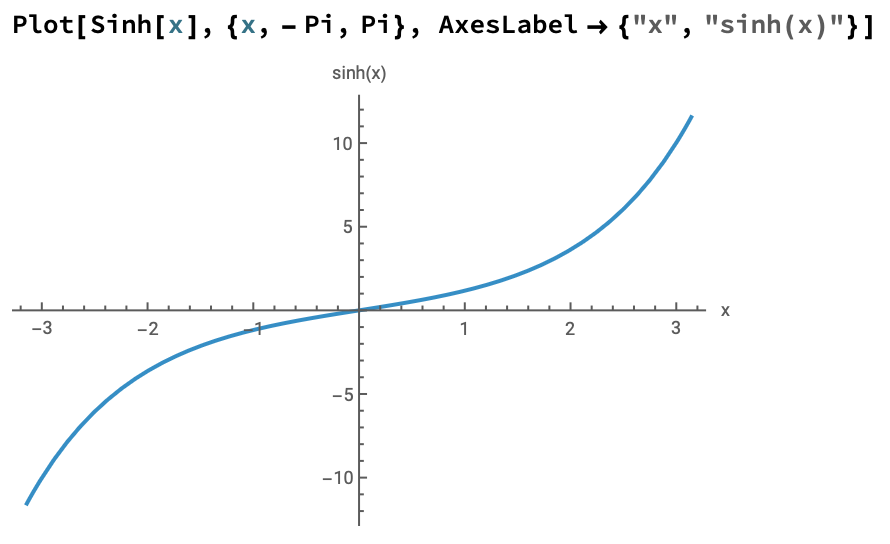
Show that \(\cosh^2z-\sinh^2z = 1\)
First, I'll square my expressions for sinh and cosh. Then I'll subtract and simplify: \begin{eqnarray*} \cosh^2z - \sinh^2z &=& \left(\frac{e^z+e^{-z}}{2}\right)^2-\left(\frac{e^z-e^{-z}}{2}\right)^2\\[6pt] &=&\frac{1}{4}\left(e^z+e^{-z}\right)^2 - \frac{1}{4}\left(e^z-e^{-z}\right)^2 \\[6pt] &=& \frac{1}{4}\left[\left(\cancel{e^{2z}}+\cancel{e^{-2z}}+2\right)- \left(\cancel{e^{2z}}+\cancel{e^{-2z}}-2\right)\right]\\[6pt] &=& \frac{4}{4}\\ &=& 1\checkmark \end{eqnarray*}
- Calculate the derivatives of \(\cosh z\) and \(\sinh z\). Do the derivatives make sense when looking at the plots of the originals functions? Explain
\begin{eqnarray*} \frac{d}{dz}\left(\sinh{z}\right) &=& \frac{d}{dz}\left(\frac{e^z-e^{-z}}{2}\right) \\[6pt] &=& \frac{e^z - (-e^{-z})}{2} \\[6pt] &=& \cosh{z}\\[6pt] \end{eqnarray*}
and \begin{eqnarray*} \frac{d}{dz}\left(\cosh{z}\right) &=& \frac{d}{dz}\left(\frac{e^z+e^{-z}}{2}\right) \\[6pt] &=& \frac{e^z+ (-e^{-z})}{2} \\[6pt] &=& \sinh{z}\\[6pt] \end{eqnarray*} These derivatives have zeroes at \(z=0\) (the local extrema of the original functions). The signs (\(\pm\)) of the derivative functions corresponds to the sign of the slope of the original functions: The slope of \(\cosh(z)\) is negative with \(z<0\) and positive when \(z>0\) (matching the sign of \(\sinh\)). The slope of \(\sinh(z)\) is always positive (matching the sign of \(\cosh\)).
- Show that \( \int \left(1/\sqrt{1+x^2}\right)dx=\mbox{arcsinh}\;x\)
(Hint: One way to do this is to make the trig substitution \(x=\sinh z\))
Using the hint given:
\(x=\sinh(z)\) and \(dx=\cosh(z)dz\) \begin{eqnarray*} \int \frac{dx}{\sqrt{1+x^2}}&=& \int \frac{\cosh(z)dz}{\sqrt{1+\sinh^2(z)}} \end{eqnarray*} Now use the trig identity: \(1+\sinh^2(z)=\cosh^2(z)\) \begin{eqnarray*} \int \frac{dx}{\sqrt{1+x^2}}&=&\int \frac{\cosh(z)dz}{\sqrt{\cosh^2(z)}}\\ &=& \int dz\\ &=& z\\ &=&\mbox{arcsinh}\;x \end{eqnarray*} Depending on the range of integration, you may need to be careful about signs when using this identity.
- Plot the behavior of \(\cosh z\) and \(\sinh z\) over a suitable range of real values z. Describe the behavior of these functions in words and note what the values of the functions are near \(z=0\) and \(z=\pm \infty\).