Contemporary Challenges: Fall-2024
Homework 1 (SOLUTION): Due 5 Friday 10/4
- Travel by car or bike
S1 5082S
(Remember to read the Homework-Write-Up Guide)
In this question you will compare the energy used by (i) an electric bicycle traveling 15 miles at 15 mph to (ii) the energy used by an electric car traveling the same distance at 60 miles per hour.
- Find the ratio of the energies used by the two options. I'm looking for a numerical value of the ratio. Use the simplest coarse-grained model for transport (kinetic energy of the wind tail) and clearly state your assumptions (for example, assume flat roads).
- Use a more refined model by including rolling resistance. The rolling resistance for cars and bicyles is equivalent to climbing an uphill grade of approximately 1%. (The exact value of the equivalent uphill grade depends on the tire pressure, and the viscoelasticity of the tire material).
As we saw in class, the energy in the wind tail of a car is given by
\begin{align*} \text{Energy in car's wind trail} &= \frac{1}{2}\rho C_{\text{D,car}} A_{\text{car}} v_{\text{car}}^2 d. \\ \end{align*}
For a bike, I can then write down
\begin{align*} \text{Energy in bike's wind trail} &= \frac{1}{2}\rho C_{\text{D,bike}} A_{\text{bike}} v_{\text{bike}}^2 d. \\ \end{align*}
The ratio of these energies is \begin{align*} \frac{\text{Energy in car's wind trail}}{\text{Energy in bike's wind trail}} = \frac{\cancel{\tfrac{1}{2}}C_{\text{D,car}}A_{\text{car}} v_{\text{car}}^2\cancel{d_{car}}}{\cancel{\tfrac{1}{2}}C_{\text{D,bike}} A_{\text{bike}} v_{\text{bike}}^2\cancel{d_{bike}}} \\ \end{align*}
since I'm considering the car and the bike going the same distance. The ratio of the speeds is 4 (given in the question prompt). As discussed in class, \(C_{\text{D,car}}A_{\text{car}} \approx 1 \text{ m}^2\). An adult riding a commuter bike presents a frontal area of about 0.5 m\(^2\) and a drag coefficient of \(\approx\) 1. Substituting these values in, I get
\begin{align*} \frac{\text{Energy in car's wind trail}}{\text{Energy in bike's wind trail}} \approx \frac{1\text{ m}^2}{0.5\text{ m}^2}(4)^2=32 \\ \end{align*}
This tells me that the car uses about 32 times more energy than the bike.
To include rolling resistance in my model, \begin{align*} \frac{E_{\text{car}}}{E_{\text{bike}}} &= \frac{\text{Energy in car's wind trail} + \text{Work done on car by rolling resistance}}{\text{Energy in bike's wind trail} + \text{Work done on bike by rolling resistance}} \\ &= \frac{\tfrac{1}{2}C_{\text{D,car}}A_{{\text{car}}} \rho_{\text{air}} v_{\text{car}}^2\cancel {d_{\text{car}}} + m_{\text{car}}g[0.01] \cancel{d_{\text{car}}}}{\tfrac{1}{2}C_{\text{D,bike}} A_{\text{bike}} \rho_{\text{air}} v_{\text{bike}}^2\cancel{d_{\text{bike}}}+ m_{bike}g [0.01]\cancel{d_{\text{bike}}}} \\ \end{align*}
Where I've modeled the rolling resistance as equivalent to climbing a 1% slope. A typical car mass might be 1500kg and a typical bike and rider mass might be 80 kg.
The density of air is \(\rho_{air} \approx 1.2 \text{ kg/m}^3\)
Making conversions to SI units: \begin{align*} v_{\text{car}} = 60 \text{ mph} \left(0.44 \frac{\text{m/s}}{\text{mph}}\right) = 26.4 \text{ m/s}\\ v_{\text{bike}} = 15 \text{ mph} \left(0.44 \frac{\text{m/s}}{\text{mph}}\right) = 6.6 \text{ m/s}\\ \end{align*}
Plugging in \begin{align*} \frac{E_{\text{car}}}{E_{\text{bike}}} &= \frac{\tfrac{1}{2}[1 \text{ m}^2] [1.2 \text{ kg/m}^3][26.4 \text{ m/s}]^2 + 0.01[1500 \text{ kg}][10 \text{ N/kg}] }{\tfrac{1}{2} [0.5 \text{ m}^2] (1.2 \text{ kg/m}^3] [6.6 \text{ m/s}]^2+ 0.01[80 \text{ kg}][10 \text{ N/kg}]} \\ &= 27 \end{align*} So, in this more realistic model, the car uses about 27 times more energy than the bicycle. Including rolling resistance refines the initial model, but the correction is relatively small.
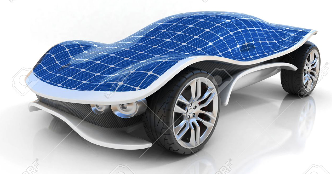
- Speed of a solar car
S1 5082S
This self-driving solar car is travelling on a flat road on a windless day. The sun is directly overhead.
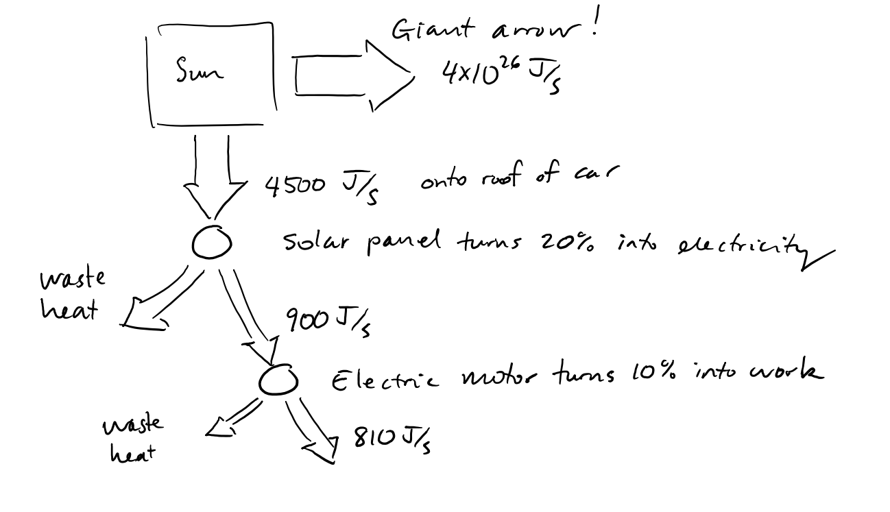
(a) Draw an energy flow diagram to describe the system. An arrow at the top of the flow diagram will represent incoming solar energy (landing on the solar panel). One circle will represent the solar panel, and one circle will represent the electric motor. Label each arrow with the correponding value of energy flow (a quantity measured in joules per second).
(b) Estimate how fast this self-driving solar car can travel on a flat road on a windless day when the sun is directly overhead. Give your answer in meters per second.
Use the following parameters for the system:
- The car is 1.8 m wide, 1 m tall and 3 m long. The top surface of the car is entirely covered with solar panels.
- The sun is directly overhead and the intensity of the sunlight is 1000 J/(s.m\(^2\)).
- The electric motors are powered directly by the solar panels (no battery power).
- The solar panels convert sunlight energy into electrical energy with 20% efficiency (the other 80% of sunlight energy is heating the solar panel).
- The electric motors convert electrical energy into mechanical work with efficiency 90% efficiency.
- The drag coefficient is 0.2.
- The energy dissipation associated with the tires rolling on the road can be neglicted.
We want to extimate how fast a new solar car design can travel.
The 810 J/s goes into the Kinetic Energy of wind behind the car. \begin{align*} \frac{KE}{\Delta t} &= 810 \text{ J/s} \\ &= \frac{\frac{1}{2} \rho_{\text{air}} C_{\text{drag}} A v^{2}d}{\Delta t}\\ &= \frac{1}{2} \rho_{\text{air}} C_{\text{drag}} A v^{2}\frac{d}{\Delta t}\\ &= \frac{1}{2} \rho_{\text{air}} C_{\text{drag}} A v^{2}v \\ &= \frac{1}{2} \rho_{\text{air}} C_{\text{drag}} A v^{3} \end{align*} In this case, \(\rho_{\text{air}} = 1.3 \text{ kg/m}^3\), \(C_{\text{drag}} = 0.2\), and \(A = 1.5 \text{ m}^2\). We can use equation 1 to solve for \(v\) and substitute in the numerical values. \begin{align*} v = \sqrt[3]{\frac{2(810 \text{ J/s})}{(1.3 \text{ kg/m}^3) (1.5 \text{ m/s}) (0.2)}} = 16 \text{ m/s} \end{align*}
Sense-making
From class, we know KE\(_\text{of air}\)/\(\Delta\)t = 20,000 J/s when driving a car at 70 mph. The solar car is going 36 mph (about half the speed) and for the solar car KE\(_\text{of air}\)/\(\Delta\)t is about 20 times less. 70 mph \(\rightarrow\) 36 mph is consistent with reducing \(v^3\) by a factor of about 8. KE\(_\text{of air}\)/\(\Delta\)t has also been reduced by aerodynamic design.
- Piano tuners in Chicago
S1 5082S
In a fabled story about Enrico Fermi (famous physicist), Fermi was asked how many people work as piano tuners in Chicago. Fermi did some mental arithmetic and quickly answered the question with surprising accuracy. Your task is to recreate Fermi's calculation.
Fermi's approach to solving such problems has spread far beyond the physics community. Today, tech companies and business consulting companies expect their employees to do Fermi problems: https://www.youtube.com/watch?v=KAo6Vn5bDF0.
Background: Pianos were popular when Fermi was living in Chicago in the 1940s. The population of Chicago was about 2 million people. Approximately 1 in 10 households had a piano. Pianos got out of tune at regular intervals (about 2 or 3 years), so the piano owner would call a technician (the piano tuner) to tighten/loosen the 88 strings inside the piano. Each tuning job took at least an hour.
Fermi used his general knowledge to estimate proportionality constants: For example, the number of pianos in Chicago was proportional to the number of households (the proporitionality constant was 0.1.).
To recreate Fermi's calculation make your own quantitaive estimates of proportionality constants (practice using your reasoning skills; avoid using Google). Each proportionality constant will be approximate; that is the essence of this estimation technique. To organize your calculation in a logical, easy-to-follow fashion, set up each line of math with one proportionality constant. For example,
\begin{align} ``(2 \times 10^6 \text{ people}) \div (3 \text{ people per household}) = 0.7 \times 10^6 \text{ households}'' \end{align}
Keep track of units as you go along: households, pianos, hours, etc. Use round numbers at each step of the calculation because a 5% calculational “error” will be smaller than the 10-30% uncertainty in the proportionality constants. How many piano tuners do you think were working in Chicago in the 1940s?
In the work below, I bold faced the five proportionality constants. I start with the population and estimate the number of households \begin{align} \text{(population of Chicago)} \div \textbf{(persons per household)} = \text{households} \end{align} Using the number of households, I calculate the number of pianos \begin{align} \text{households} \div \textbf{(households per piano)} = \text{pianos} \end{align} Using the number of pianos, I calculate the number of tunings per year, \begin{align} \text{pianos} \times \textbf{(tunings per piano per year)} = \text{tunings per year} \end{align} I need to know how many tunings a technician can perform each year: \begin{align} \textbf{(hours per technician per year)} \div \textbf{(hours per tuning)} = \text{tunings per technician per year} \end{align} Finally, I can calculate the number of technicians, \begin{align} \text{tunings per year} \div \text{tunings per technician per year} = \text{technicians} \end{align} Let's put in some numbers. Well assume a population of 2 million people. A typical household in the US is probably one kid and two parents (3 people), so there are \(\sim\)0.7 million households in Chicago.
The fraction of households that have a piano is less than 100% and probably more than 1%. I'll guess 10%. That means about 70,000 pianos in Chicago.
How often do people tune pianos? They shouldn't wait 10 years, but they can't afford every month. I'll guess once per year. Therefore, we expect 70,000 tuning jobs per year. (Note by David Roundy: I think we've had our piano tuned twice in 15 years, so this is perhaps a bit optimistic.)
It probably takes more than 1 hour to tune a piano but less than 10 hours (there are 88 keys and it probably takes about a minute for each string). I'll guess it takes 2 hours.
A typical worker works 40 hours/week \(\approx\)2000 hours/year. That means one technician can tune 1000 pianos per year. In conclusion, there must be about 70 piano tuners in Chicago.
Note: There are absolutely other ways you could have solved this problem had we not asked you to estimate hours. You could instead have estimated the salary of a piano tuner and the cost of a piano tuning. That's probably harder, if you've never paid to have your piano tuned.
- Three ideas for the term project
S1 5082S
Read the description of the term project on the class website at “Introduction to term project”. Identify three (3) subjects that you find interesting/intriguing (for example, solar energy, exoplanets, ...). Within each subject, pose a question that might have an interesting quantitative answer: “Since it requires energy to make a solar panel, how long does it take to recoup that energy?”, “How far away could we see an Earth-like planet orbiting a Sun-like star?” ... You should turn in 3 different subjects and 3 different quantitative questions (quantitative means “quantities that can be calculated and/or measured”)
Let your mind wander as broadly as possible. Subjects and questions are not restricted to the topics taught in PH315. During this exploratory stage, be bold and daring; you are not committing yourself to solve all 3 questions. To spark your imagination, there is a list of ideas on the class website. The instructor will read your ideas and give you feedback. Whenever possible, the feedback will point you towards a coarse-grained model that is helpful for answering your question. Use the feedback to help decide which question you will develop further (or whether you need to go back to the drawing board).
Here are some general comments which the instructor might reference when giving individual feedback.
Cost estimates
General advice: If an accountant could solve your question, you haven't included enough physics.
There are important/interesting relationships between physics and what stuff costs. For example, if you understand the rocket equation, and you know the price of rocket fuel, you can set a minimum cost for launching payloads into space. The cost of launching payloads into space is a great example of how we can connect physics to the real world. However, please keep the physics in your question/solution and avoid focusing exclusively on tallying up dollar amounts.Topics in alphabetical order
Airplane flight: The textbook "Sustainable Energy Without the Hot Air" gives some excellent models about airplane energy consumption (see the technical appendices that explain the mathematical models at the end of the book). These models allow you to explore the effect of changing the weight and velocity of the aircraft, as well as the effect of changing the air density or even the force of gravity (flight on Mars?).
Cars and delivery trucks: The energy used for stop-and-go driving can be described by a coarse grain model. See MacKay textbook for details. Differences in operating cost between gas-powered cars and electric cars are interesting. Note that city driving (coarse-grained model) is strongly affected by vehicle weight, but highway driving is nearly independent of vehicle weight (except for rolling resistance).
Desalination: There is a simple physical model to calculate the energy required to desalinate water. The work done is PdV, just like gas processes. The osmotic pressure, P, can be written in the same form as the ideal gas law, PV = nRT, where n is the number of moles of solute molecules. Despite being different physical systems (one is a gas, the other is salt dissolved in water), they share the same mathematical description because the entropy of the solute molecules in liquid is identical to the entropy of gas molecules in an ideal gas. The entropy explanation for osmotic pressure is a bit abstract. Therefore, it's interesting to think about a physical model of what happens on the microscopic level. How would the salt water interact with a semipermeable membrane? Here is a link to such a model: “OSMOSIS: A MACROSCOPIC PHENOMENON, A MICROSCOPIC VIEW” https://journals.physiology.org/doi/full/10.1152/advan.00015.2002
Direct-Air-Capture of CO2: You could make a physical model of direct-air capture of CO2. You have to blow air across the surface of water. CO2 can dissolve in water. Chemicals in the water can bind to the dissolved CO2. The tricky part of the calculation is finding the work done driving laminar air flow through a constricted space. Learn about the viscosity of air and the physics of laminar flow. Useful comparisons include: How much CO2 does a tree capture? How much CO2 does seaweed capture?
Drones, Helicopters, Honeybees and Humming Birds: There is a coarse-grain model to figure out how much energy it takes for a flying vehicle to hover in mid-air. The spinning blades (or honeybee wings) generate a downdraft. This downward moving air has momentum. The rate of momentum generation (kg.m/s per second) is equal to the force that counteracts gravity. Once you do the momentum calculation, you can then figure out energy used: \(\frac{1}{2}mv^2\), where \(m\) is the mass of air used in the downdraft, and \(v\) is the velocity of the downdraft.
Earth-like planets in the Milky Way galaxy: The Drake equation is a popular way to estimate whether life exists outside our solar system (there is a good Wikipedia page about the Drake equation). You can use a simple climate model (from Unit T) to estimate the range of orbital distances that yield a good planet temperature near a sun-like star. This adds some interesting physics to the calculation of probabilities that enter the Drake equation. Also, there is always new data to consider about earth-like planets. For example: https://www.universetoday.com/146583/astronomers-estimate-there-are-6-billion-earth-like-planets-in-the-milky-way/.
Energy used by a Data Center: It's interesting to think about the energy a computer uses to process information. You need a course-grain model of the physical process used inside computers. At the heart of a computer are MOSFETs (a type of transistor). A MOSFET is a parallel plate capacitor (the channel is one plate, the gate is the other plate). There are about 1 billion transistors in a processor. Some fraction of them switch every cycle (1 GHz cycling rate?). When a transistor switches, it dumps the energy stored in the capacitance \(\frac{1}{2}CV^2\). https://www.intel.com/pressroom/kits/core2duo/pdf/epi-trends-final2.pdf .
Fluid flow in pipes: Hagen-Poiseuille equation allows you to develop simple models for the work done moving liquid along a pipe.
Food production: For each type of crop, you can look up an efficiency fraction = (food energy)/(solar energy). There are maps of solar energy as function of location and month. For data on Oregon, I like this website: http://solardat.uoregon.edu/NorthwestSolarResourceMaps.html.
Food consumption: Humans eat food and utilize that chemical energy at a rate of about 80 J/s. In the United States, humans use their other sources of energy at an average rate of about 8000 J/s. It's a big difference! There are multiple course-grained methods to estimate the rate 80 J/s. This can be an excellent topic for the term project. Course-grain methods include (i) radiative heat transfer to the environment, (ii) food consumption, (iii) the volume of air we breathe. (The oxygen we consume is used to "burn" carbohydrates and power our bodies...)
General Relativity: The wikipedia page on "gravitational redshift" discusses some historical controversy that could make good material for a question. It is possible to estimate the Schwarzschild radius by simple methods (see class notes) Video by minute physics: "the unreasonable efficiency of black holes": https://www.youtube.com/watch?v=t-O-Qdh7VvQ. Heat transfer (e.g. temperature of a spaceship) In many cases you can ignore convective heat transfer and just focus on radiative heat transfer. Radiative heat transfer models give lots of insight and are easier to implement mathematically than convective heat transfer. See UnitT6.4 for some guidance about the Stefan-Boltzmann law, and example questions at the end of the chapter such as T6M.4. Radiative heat transfer explains how a spaceship or satellite maintains a steady temperature. Radiative heat transfer gives a good estimate for energy consumed by a human.
Heat transfer (e.g. heating a meteorite from the outside): The heat equation is a PDE with so many useful applications. https://en.wikipedia.org/wiki/Heat_equation The university education of an engineer can involve years studying all the different approaches to solving this equation. In the context of this class, we need a quick first-order (approximate) analysis. A general approach that I recommend: imagine your system as slabs of finite thickness and uniform temperature. For example, a sphere heated from the center might be modelled like the layers of an onion. Energy flows from hotter slabs to colder slabs. Before the system reaches steady state, the transient behavior might be tricky to model. You'd have to take finite time steps and use a program like excel, matlab or python to help you. When the system reaches steady state, the math should get easier.
Hydroelectric power: Questions about hydroelectric can be “rich context” if you apply to a specific situation. For example, you might start with basic info like the annual rainfall and catchment area of the river, and compare to the population and per capita energy consumption. For making a simple model (including things like rainfall catchments), there is guidance in the "Sustainable Energy Without the Hot Air".
Hyperloop: The hyperloop concept is a nice system to analyze. There are good resources available on the internet. There are multiple questions you can ask. For example, how the energy usage scales with air pressure inside the tube, what are the concerns about making the system safe, how much energy is used to maintain the vacuum.
Ionizing radiation (alpha, beta and gamma radiation): Chpt 15 of Unit Q discusses some physical models of biological effects of radiation. I've also written a question along these lines, which I'd be happy to share as a starting point. Maximum dose needed for medical imaging is another interesting angle to think about.
Information technology: About 5% of electricity in the US is being used for data centers, computers, internet, streaming data etc. Interesting coarse grain models include energy used per bit of information transmitted down a fiberoptic cable, and the energy used to process one bit of information using a modern integrated circuit. https://www.intel.com/pressroom/kits/core2duo/pdf/epi-trends-final2.pdf .
Laser weapons: https://en.wikipedia.org/wiki/Laser_weapon Wikipedia as a detailed overview, including a chart describing over 50 military projects/experiments. The Locust system is the most recent in 2026.
Methane as a greenhouse gas: To calculate the potency of methane, you'll need to consider the current concentration of methane in the atmosphere, and calculate the optical pathlength for IR light that is resonant with methane vibrations. If you feel comfortable with such calculations, this would be a great question. The MODTRAN atmosphere simulator will also be helpful. I have class-notes from week 9 that will be helpful (happy to share them with you).
Oceans: Energy from temperature differences in Ocean: There is a small OTEC plant operating in Hawaii (OTEC = ocean thermal energy conversion plant. As a physicist you can do a zeroth-order analysis of this specific system and then start asking questions like: would the system work in Oregon?; can the system be scaled up?; what is the energy cost of making the cold-water intake deeper in the ocean?
The heat engine in an OTEC plant uses ammonia as the working gas and takes heat from a hot reservoir (warm water) and dumps heat into a cold reservoir (cold water). Please don't get bogged down in trying to learn how engineers build a closed-loop ammonia system and how expanding ammonia gas is used to do work on a turbine (the turbine replaces the piston we discussed in class). It takes years of engineering school to design the inner workings of an industrial heat engine. If you are worried about fine tuning your calculation, you can always change this “engineering factor” from 70% of Carnot efficiency to 80% of Carnot efficiency or vice versa.
Neutron stars: Some of the concepts that are covered in the nuclear physics section of the course are relevant for analyzing neutron stars.
Pulsars: The mechanism of pulsar luminosity hasn't been figured out yet. However, there are still fun calculations related to pulsars. We know that a pulsar is a spinning object and a pulse from a pulsar happens every 5 milliseconds or so. What is the maximum radius of an object that is spins this fast yet is still held together by gravity? Can we put limits on the mass density of a pulsar?
Quantum Computing: It's difficult to explore quantum computing without learning a lot more quantum mechanics and the associated mathematical language/techniques. However, there are accessible entry points. Physicists like Nicolas Gisin have developed wonderful and insightful back-of-the-envelop calculations related to Bell's theorem. I recommend reading Jeffery Bub's most recent book “Totally Random” (or his earlier book “Bananaworld”). Both e-book versions are available from OSU library. Bub describes a pair of entangled quantum coins that produce correlated coin toss results. You could write a homework question related to Bub's proof that the quantum coins cannot be rigged to mimic the observed entanglement correlation. “Totally Random” also explains a number of applications for quantum entanglement which are accessible to PH315 students. Please note that entanglement is the true resource required for quantum computing to outperform classical computing. Therefore, a solid understanding of entanglement is a critical first step before understanding quantum computing.
Quantum Mechanics applied to Astrophysics: It's possible to estimate the Chandrasekhar mass by fairly simple methods (see wikipedia article). Chandrasekhar mass is the largest mass for a stable white dwarf, it is governed by the pressure it takes to squeeze an electron into a small space (compressing the deBroglie wavelength to very small size). Similar physics goes into calculating the largest possible mass of a neutron star (squeezing the deBroglie wavelength of neutrons). People argue about the exact upper limit to the neutron star's mass because you have to consider how general relativity interacts with quantum mechanics. This gets complicated!
Sky Hooks and Space Elevators: The term project webpage has links to YouTube video about sky hooks (space tethers). A word of caution, however. In past years, students have struggled with space tethers because it's hard to simplify the calculations. The equations get messy very quickly. It's hard to design a simple thought experiment to illustrate how the proposed systems will work. I haven't found good resources to guide students beyond the superficial YouTube video.
Solar power in Oregon: There are some great maps of oregon solar energy at this website: http://solardat.uoregon.edu/NorthwestSolarResourceMaps.html. If you write an Oregon solar energy question, consider referring to these maps in your question. Space travel: laser-powered sail An important challenge is the divergence of the laser beam. You should look at Figure Q3.9 "A graph of intensity vs. sin(theta) for waves going through a single slit..." The accompanying text is "Q3.5 Diffraction Revisited".
Space travel: rockets: Take a look at "the rocket equation" (Wikipedia). If you are mostly concerned with escaping Earth's gravity, you'll also need to read about escape velocity on Wikipedia. Using today's technology, the launch mass of a rocket is mostly rocket fuel... the payload is only a small fraction. Also, note that the amount of energy required for space travel depends on the propulsion system (mass of the propellent, velocity of the propellent).
Space travel: changing orbit: If you want to move a heavy object into a different orbit, you'll need a detailed step-by-step plan. It's not satisfactory to simply say “I'll magically change the gravitational potential energy and the kinetic energy”. For a specific step-by-step plan, consider using the Hohmann transfer orbit: https://en.wikipedia.org/wiki/Hohmann_transfer_orbit or you can compare Hohmann to something else. If you want to calculate the energy required, please remember that the amount of energy required to move something by rocket propulsion depends on the propulsion system.
Superconductors at high pressure: This is an exciting topic. Here is an article about recent advances in the research field: https://www.nature.com/articles/d41586-020-02895-0. The prediction by Neil Ashcroft is very relevant. He noted that hydrogen (pressed into solid form) is the best choice for getting superconductivity at room temperature (because hydrogen is light weight and it has a half-filled electron shell). You could look up Ashcroft's prediction/equations and try to write your question about it.
Stars: The rate of energy emission (electromagnetic radiation) from a star can be calculated from the Stefan-Boltzmann law if you know the star's surface temperature and radius. See UnitT6.4 for some guidance about the Stefan-Boltzmann law.
Transmission line energy loss: Estimating the energy loss over transmission lines is a good question. Some transmission is done at 200 kV, some at 50 kV, how thick are the cables? how long are the cables? What fraction of the energy transmitted is wasted?
Wind: The internet has useful maps showing the average wind speed around the United States. https://windexchange.energy.gov/maps-data/325
Wireless power transmission (far-field techniques): Read about wireless power transfer on Wikipedia, especially the subsection about far-field techniques. You should be able to calculate the size of the transmitting antenna and the receiving antenna for a given situation. The textbook Unit Q will help you understand the main physics concepts. See Figure Q3.9 A graph of intensity versus sin(theta) for waves going through a slit.